"""
Examples of using the GOL plotting functions.
"""
import numpy as np
from srxraylib.plot.gol import *
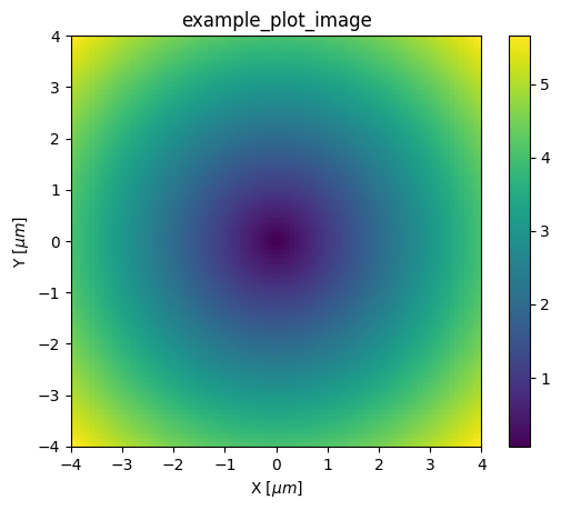
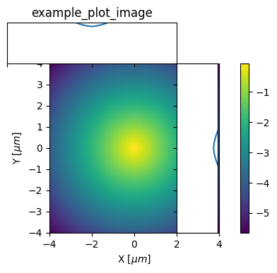
def example_plot_image():
x = np.linspace(-4, 4, 90)
y = np.linspace(-4, 4, 90)
print('Size %d pixels' % (len(x) * len(y)))
z = np.sqrt(x[np.newaxis, :]**2 + y[:, np.newaxis]**2)
plot_image(z,x,y,title="example_plot_image",xtitle=r"X [$\mu m$]",ytitle=r"Y [$\mu m$]",cmap=None,show=1)
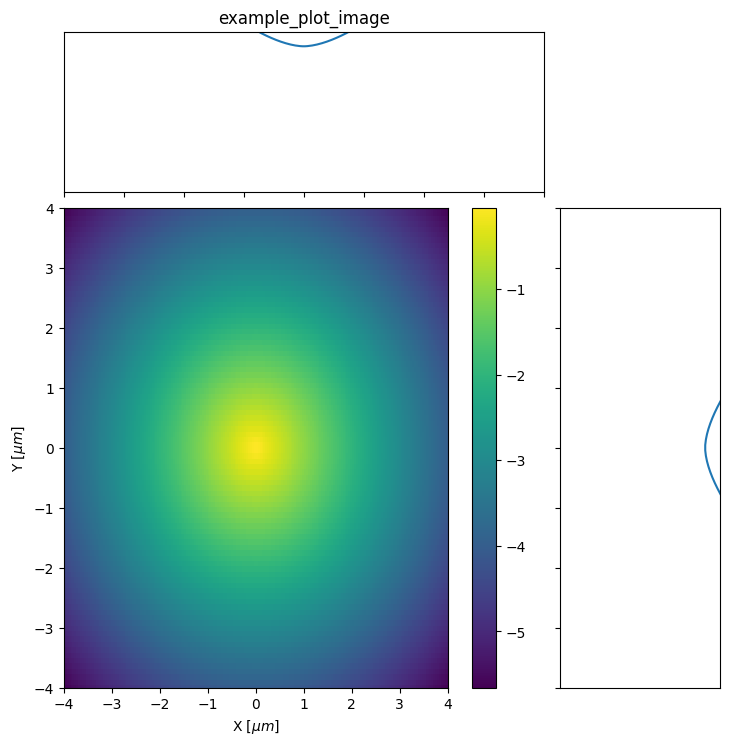
def example_plot_image_with_histograms():
x = np.linspace(-4, 4, 200)
y = np.linspace(-4, 4, 90)
print('Size %d pixels' % (len(x) * len(y)))
z = -np.sqrt(x[np.newaxis, :]**2 + y[:, np.newaxis]**2)
plot_image_with_histograms(z.T,x,y,title="example_plot_image",xtitle=r"X [$\mu m$]",ytitle=r"Y [$\mu m$]",
cmap=None,show=1,figsize=(8,8),add_colorbar=True)
plot_image_with_histograms(z.T, x, y, title="example_plot_image", xtitle=r"X [$\mu m$]", ytitle=r"Y [$\mu m$]",
cmap=None, show=1, figsize=(10,4), aspect='equal', add_colorbar=True)
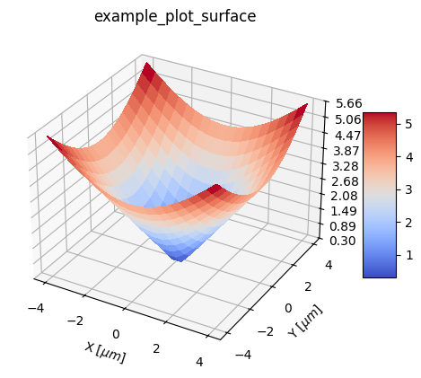
def example_plot_surface():
x = np.linspace(-4, 4, 20)
y = np.linspace(-4, 4, 20)
print('Size %d pixels' % (len(x) * len(y)))
z = np.sqrt(x[np.newaxis, :]**2 + y[:, np.newaxis]**2)
plot_surface(z,x,y,title="example_plot_surface",xtitle=r"X [$\mu m$]",ytitle=r"Y [$\mu m$]",cmap=None,show=1)
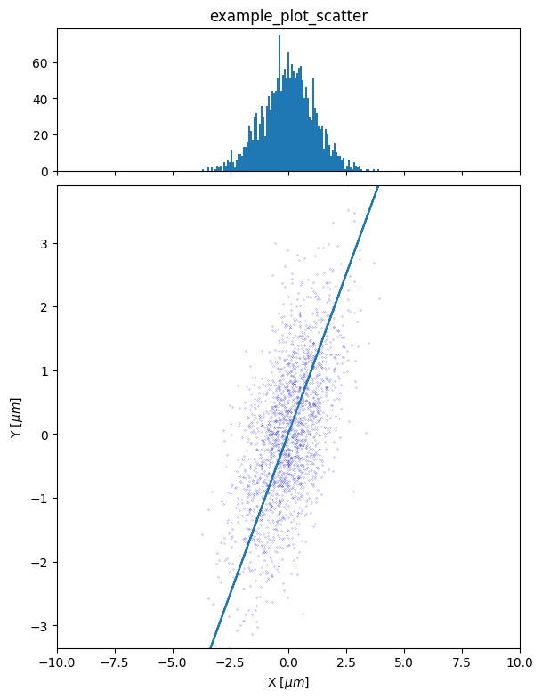
def example_plot_scatter():
#example motivated by http://www.ster.kuleuven.be/~pieterd/python/html/core/scipystats.html
from scipy import stats
# x = np.random.rand(1000)
# y = np.random.rand(1000)
x = stats.norm.rvs(size=2000)
y = stats.norm.rvs(scale=0.5, size=2000)
data = np.vstack([x+y, x-y])
f = plot_scatter(data[0],data[1],xrange=[-10,10],title="example_plot_scatter",
xtitle=r"X [$\mu m$]",ytitle=r"Y [$\mu m$]",plot_histograms=2,show=0)
f[1].plot(data[0],data[0]) # use directly matplotlib to overplot
plot_show()
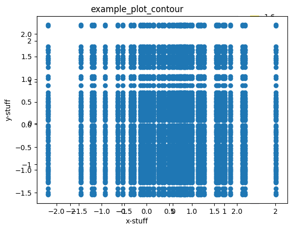
def example_plot_contour():
# deprecated in matplotlib. Copied from" https://github.com/matplotlib/matplotlib/blob/81e8154dbba54ac1607b21b22984cabf7a6598fa/lib/matplotlib/mlab.py#L1866
def bivariate_normal(X, Y, sigmax=1.0, sigmay=1.0,
mux=0.0, muy=0.0, sigmaxy=0.0):
"""
Bivariate Gaussian distribution for equal shape *X*, *Y*.
See `bivariate normal
<http://mathworld.wolfram.com/BivariateNormalDistribution.html>`_
at mathworld.
"""
Xmu = X - mux
Ymu = Y - muy
rho = sigmaxy / (sigmax * sigmay)
z = Xmu ** 2 / sigmax ** 2 + Ymu ** 2 / sigmay ** 2 - 2 * rho * Xmu * Ymu / (sigmax * sigmay)
denom = 2 * np.pi * sigmax * sigmay * np.sqrt(1 - rho ** 2)
return np.exp(-z / (2 * (1 - rho ** 2))) / denom
# inspired by http://stackoverflow.com/questions/10291221/axis-limits-for-scatter-plot-not-holding-in-matplotlib
# random data
x = np.random.randn(50)
y = np.random.randn(100)
X, Y = np.meshgrid(y, x)
Z1 = bivariate_normal(X, Y, 1.0, 1.0, 0.0, 0.0)
Z2 = bivariate_normal(X, Y, 1.5, 0.5, 1, 1)
Z = 10 * (Z1 - Z2)
plot_contour(Z,x,y,title='example_plot_contour',xtitle='x-stuff',ytitle='y-stuff',plot_points=1,show=1)
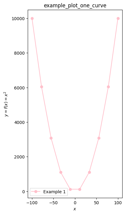
def example_plot_one_curve():
x = np.linspace(-100,100,10)
y = x**2
plot(x,y,xtitle=r'$x$',title="example_plot_one_curve",
ytitle=r'$y=f(x)=x^2$',legend="Example 1",color='pink',marker='o',linestyle=None,
figsize=(4,8),show=1)
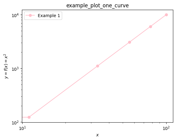
def example_plot_one_curve_log():
x = np.linspace(-100,100,10)
y = x**2
plot(x,y,xtitle=r'$x$',title="example_plot_one_curve",
ytitle=r'$y=f(x)=x^2$',legend="Example 1",color='pink',marker='o',linestyle=None,xlog=1,ylog=1,show=1)
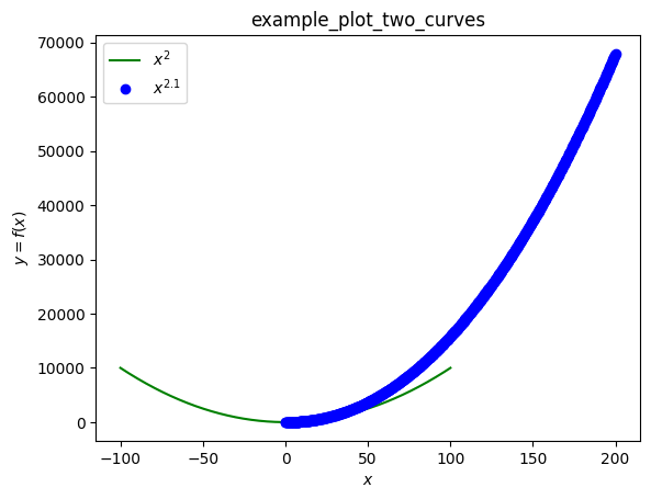
def example_plot_two_curves():
x1 = np.linspace(-100,100,1000)
y1 = x1**2
x2 = np.linspace(0,200,700)
y2 = x2**2.1
plot(x1,y1,x2,y2,xtitle=r'$x$',title="example_plot_two_curves",
ytitle=r'$y=f(x)$',legend=[r"$x^2$",r"$x^{2.1}$"],color=['green','blue'],marker=[' ','o'],linestyle=['-',' '],show=1)
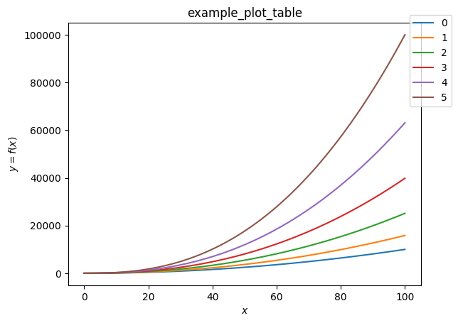
def example_plot_table():
x1 = np.linspace(0,100,100)
out = np.zeros((6,x1.size))
out[0,:] = x1**2
out[1,:] = x1**2.1
out[2,:] = x1**2.2
out[3,:] = x1**2.3
out[4,:] = x1**2.4
out[5,:] = x1**2.5
# another way
# out = np.vstack( (
# x1**2,
# x1**2.1,
# x1**2.2,
# x1**2.3,
# x1**2.4,
# x1**2.5 ))
legend=np.arange(out.shape[0]).astype("str")
plot_table(x1,out,xtitle=r'$x$',ytitle=r'$y=f(x)$',title="example_plot_table",legend=legend,show=1)
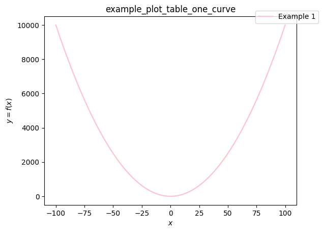
def example_plot_table_one_curve():
x1 = np.linspace(-100,100,1000)
out = x1**2
plot_table(x1,out,title="example_plot_table_one_curve",xtitle=r'$x$',ytitle=r'$y=f(x)$',legend="Example 1",color='pink',show=1)
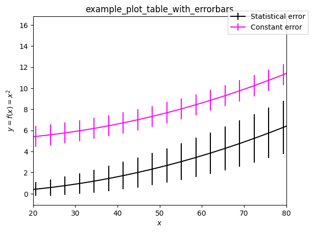
def example_plot_table_with_errorbars():
x = np.linspace(0,100,30)
out = np.zeros((2,x.size))
out[0,:] = 1e-3 * x**2
out[1,:] = 5 + 1e-3 * x**2
yerr = np.sqrt(out)
yerr[1,:] = 1.0
plot_table(x,out,errorbars=yerr,title="example_plot_table_with_errorbars",xtitle=r'$x$',ytitle=r'$y=f(x)=x^2$',xrange=[20,80],
legend=["Statistical error","Constant error"],color=['black','magenta'],show=1)
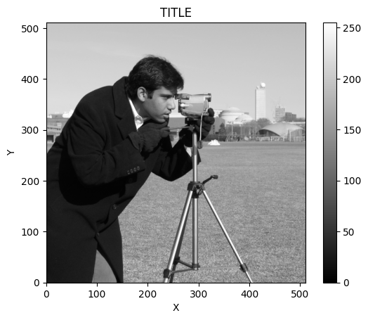
def example_plot_image_ascent():
# scipy.misc.ascent was removed in scipy 2.0; use skimage.data.camera() instead
try:
from skimage.data import camera
img = camera()
except ImportError:
img = np.random.randint(0, 256, (512, 512), dtype=np.uint8)
img = np.rot90(img, -1)
plot_image(img, np.arange(0, img.shape[0]), np.arange(0, img.shape[1]), cmap='gray')
#
# main
#
if __name__ == "__main__":
# set_qt()
# pass
example_plot_one_curve()
example_plot_two_curves()
example_plot_one_curve_log()
example_plot_table()
example_plot_table_one_curve()
example_plot_table_with_errorbars()
example_plot_image()
example_plot_image_with_histograms()
example_plot_surface()
example_plot_contour()
example_plot_scatter()
example_plot_image_ascent()