"""
Examples of calculations of synchrotron emission (radiation and angle distributions) using the functions in srfunc.
"""
import numpy
import matplotlib.pylab as plt
import scipy.constants as codata
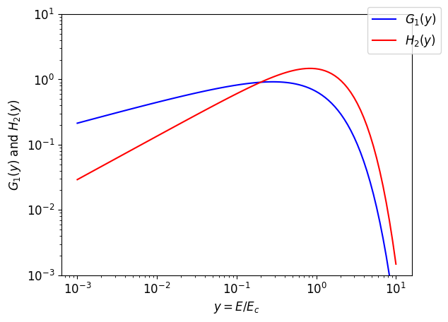
def check_xraybooklet_fig2_1(pltOk=False):
from srxraylib.sources.srfunc import sync_g1, sync_hi
print("# ")
print("# example 1, Fig 2-1 in http://xdb.lbl.gov/Section2/Sec_2-1.html ")
print("# ")
y = numpy.logspace(-3,1,100) # from 0.001 to 10, 100 points
g1 = sync_g1(y,polarization=0)
h2 = sync_hi(y,i=2,polarization=0)
# TODO: check transpose
h2 = h2.T
toptitle = "" # "Synchrotron Universal Functions $G_1$ and $H_2$"
xtitle = "$y=E/E_c$"
ytitle = "$G_1(y)$ and $H_2(y)$"
#pltOk = 0
if pltOk:
import matplotlib
font = {
# 'family': 'normal',
# 'weight': 'bold',
'size': 12}
matplotlib.rc('font', **font)
plt.figure(1)
plt.loglog(y,g1,'b',label="$G_1(y)$")
plt.loglog(y,h2,'r',label="$H_2(y)$")
plt.title(toptitle)
plt.xlabel(xtitle)
plt.ylabel(ytitle)
plt.ylim((1e-3,10))
ax = plt.subplot(111)
ax.legend(bbox_to_anchor=(1.1, 1.05))
plt.savefig('fig_universal_functions.pdf')
else:
print("\n\n\n\n\n######### %s ######### "%(toptitle))
print("\n %s %s "%(xtitle,ytitle))
for i in range(len(y)):
print(" %f %e %e "%(y[i],g1[i],h2[i]))
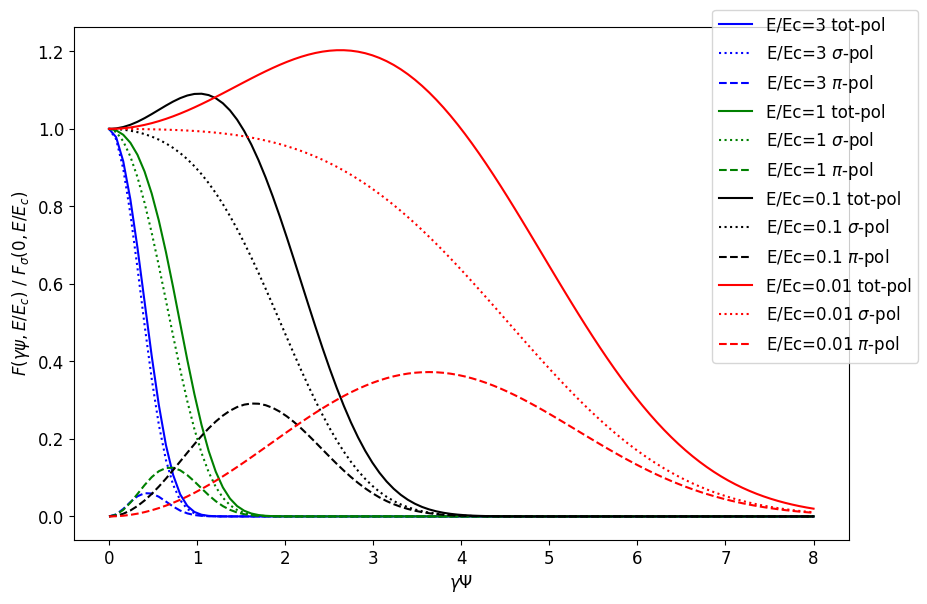
def check_xraybooklet_fig2_2(pltOk=False):
from srxraylib.sources.srfunc import sync_f
print("# ")
print("# example 2, Fig 2-2 in http://xdb.lbl.gov/Section2/Sec_2-1.html ")
print("# ")
y = numpy.linspace(0,8,100) # from 0.001 to 10, 100 points
f3 = sync_f(y, 3.0, polarization=1)
f3pi = sync_f(y, 3.0, polarization=2)
f1 = sync_f(y, 1.0, polarization=1)
f1pi = sync_f(y, 1.0, polarization=2)
fp1 = sync_f(y, 0.1, polarization=1)
fp1pi = sync_f(y, 0.1, polarization=2)
fp01 = sync_f(y, 0.01, polarization=1)
fp01pi = sync_f(y, 0.01, polarization=2)
toptitle = "Synchrotron Angular Emission"
xtitle = "$\gamma \Psi$"
ytitle = "$F(\gamma\psi, E/E_c)$ / $F_\sigma(0, E/E_c)$"
f3.shape = -1
f3pi.shape = -1
f3max = f3.max()
f1.shape = -1
f1pi.shape = -1
f1max = f1.max()
fp01.shape = -1
fp01pi.shape = -1
fp01max = fp01.max()
fp1.shape = -1
fp1pi.shape = -1
fp1max = fp1.max()
plt_total = 1
if pltOk:
import matplotlib
font = {
# 'family': 'normal',
# 'weight': 'bold',
'size': 14}
plt.figure(2, figsize=(10,6.66))
if plt_total: plt.plot(y, (f3+f3pi) / f3max, color='b', linestyle='solid', label="E/Ec=3 tot-pol")
plt.plot(y, f3/f3max, color='b', linestyle='dotted', label="E/Ec=3 $\sigma$-pol")
plt.plot(y, f3pi/f3max, color='b', linestyle='dashed', label="E/Ec=3 $\pi$-pol")
if plt_total: plt.plot(y, (f1 + f1pi) / f1max, color='g', linestyle='solid', label="E/Ec=1 tot-pol")
plt.plot(y, f1/f1max, color='g', linestyle='dotted', label="E/Ec=1 $\sigma$-pol")
plt.plot(y, f1pi/f1max, color='g', linestyle='dashed', label="E/Ec=1 $\pi$-pol")
#
if plt_total: plt.plot(y, (fp1 + fp1pi) / fp1max, color='k', linestyle='solid', label="E/Ec=0.1 tot-pol")
plt.plot(y, fp1/fp1max, color='k', linestyle='dotted', label="E/Ec=0.1 $\sigma$-pol")
plt.plot(y, fp1pi/fp1max, color='k', linestyle='dashed', label="E/Ec=0.1 $\pi$-pol")
#
if plt_total: plt.plot(y, (fp01 + fp01pi) / fp01max, color='r', linestyle='solid', label="E/Ec=0.01 tot-pol")
plt.plot(y, fp01/fp01max, color='r', linestyle='dotted', label="E/Ec=0.01 $\sigma$-pol")
plt.plot(y, fp01pi/fp01max, color='r', linestyle='dashed', label="E/Ec=0.01 $\pi$-pol")
# plt.title(toptitle)
plt.xlabel(xtitle)
plt.ylabel(ytitle)
ax = plt.subplot(111)
ax.legend(bbox_to_anchor=(1.1, 1.05))
plt.savefig('fig_angular_emission_integrated.pdf')
else:
print("\n\n\n\n\n######### %s ######### "%(toptitle))
print("\n %s %s "%(xtitle,ytitle))
for i in range(len(y)):
print(" %f %e %e "%(y[i],f3[i],f3pi[i]))
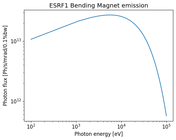
def check_esrf_bm_spectrum(pltOk=False):
from srxraylib.sources.srfunc import sync_ene
print("#")
print("# example 3, ESRF1 BM spectrum")
print("#")
# input for ESRF1
e_gev = 6.04 # electron energy in GeV
r_m = 25.0 # magnetic radius in m
i_a = 0.2 # electron current in A
# calculate critical energy in eV
codata_mee = 1e-6 * codata.m_e * codata.c ** 2 / codata.e
m2ev = codata.c * codata.h / codata.e # lambda(m) = m2eV / energy(eV)
gamma = e_gev*1e3/codata_mee
ec_m = 4.0*numpy.pi*r_m/3.0/numpy.power(gamma,3) # wavelength in m
ec_ev = m2ev/ec_m
energy_ev = numpy.linspace(100.0,100000.0,99) # photon energy grid
f_psi = 0 # flag: full angular integration
flux = sync_ene(f_psi,energy_ev,ec_ev=ec_ev,polarization=0, \
e_gev=e_gev,i_a=i_a,hdiv_mrad=1.0, \
psi_min=0.0, psi_max=0.0, psi_npoints=1)
toptitle = "ESRF1 Bending Magnet emission"
xtitle = "Photon energy [eV]"
ytitle = "Photon flux [Ph/s/mrad/0.1%bw]"
if pltOk:
plt.figure(3)
plt.loglog(energy_ev,flux)
plt.title(toptitle)
plt.xlabel(xtitle)
plt.ylabel(ytitle)
else:
print("\n\n\n\n\n######### %s ######### "%(toptitle))
print("\n %s %s "%(xtitle,ytitle))
for i in range(len(flux)):
print(" %f %12.3e"%(energy_ev[i],flux[i]))
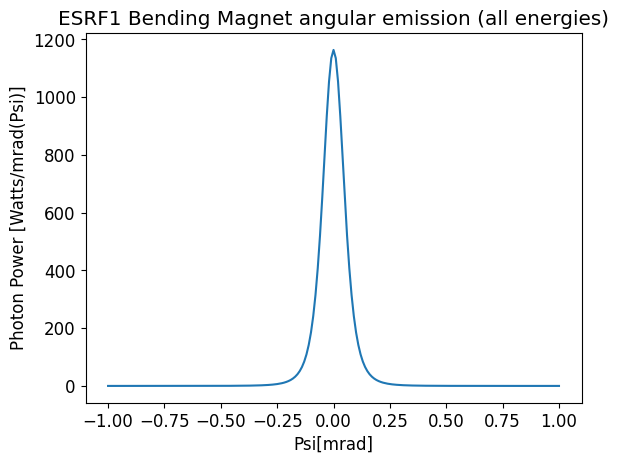
def check_esrf_bm_angle_power(pltOk=False):
from srxraylib.sources.srfunc import sync_ang
print("#")
print("# example 4: ESRF1 BM angular emission of power")
print("#")
# input for ESRF1
e_gev = 6.04 # electron energy in GeV
r_m = 25.0 # magnetic radius in m
i_a = 0.2 # electron current in A
angle_mrad = numpy.linspace(-1.0,1.0,201) # angle grid
flag = 0 # full energy integration
flux = sync_ang(flag,angle_mrad,polarization=0, \
e_gev=e_gev,i_a=i_a,hdiv_mrad=1.0,r_m=r_m)
#TODO: integrate curve and compare with total power
toptitle = "ESRF1 Bending Magnet angular emission (all energies)"
xtitle = "Psi[mrad]"
ytitle = "Photon Power [Watts/mrad(Psi)]"
if pltOk:
plt.figure(4)
plt.plot(angle_mrad,flux)
plt.title(toptitle)
plt.xlabel(xtitle)
plt.ylabel(ytitle)
else:
print("\n\n\n\n\n######### %s ######### "%(toptitle))
print("\n %s %s "%(xtitle,ytitle))
for i in range(len(flux)):
print(" %f %f"%(angle_mrad[i],flux[i]))
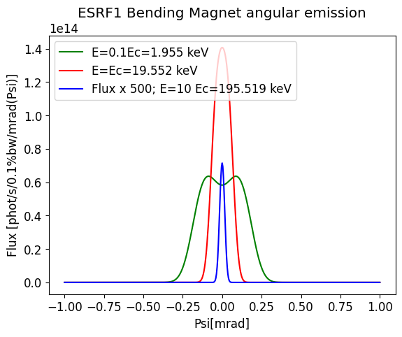
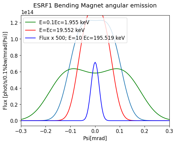
def check_esrf_bm_angle_flux(pltOk=False, method=1):
from srxraylib.sources.srfunc import sync_ang, sync_ene, sync_f
print("#")
print("# example 5: ESRF1 BM angular emission of flux")
print("#")
# input for ESRF1
e_gev = 6.04 # electron energy in GeV
r_m = 25.0 # magnetic radius in m
i_a = 0.2 # electron current in A
# calculate critical energy in eV
codata_mee = 1e-6 * codata.m_e * codata.c ** 2 / codata.e
m2ev = codata.c * codata.h / codata.e # lambda(m) = m2eV / energy(eV)
gamma = e_gev*1e3/codata_mee
ec_m = 4.0*numpy.pi*r_m/3.0/numpy.power(gamma,3) # wavelength in m
ec_ev = m2ev/ec_m
npoints = 501
angle_mrad = numpy.linspace(-1.0, 1.0, npoints) # angle grid
flag = 1 # at at given energy
polarization = 0
if method ==0:
fluxEc = sync_ang(flag,angle_mrad,polarization=polarization, \
e_gev=e_gev,i_a=i_a,hdiv_mrad=1.0,energy=ec_ev, ec_ev=ec_ev)
flux10Ec = sync_ang(flag,angle_mrad,polarization=polarization, \
e_gev=e_gev,i_a=i_a,hdiv_mrad=1.0,energy=10*ec_ev, ec_ev=ec_ev)
fluxp1Ec = sync_ang(flag,angle_mrad,polarization=polarization, \
e_gev=e_gev,i_a=i_a,hdiv_mrad=1.0,energy=0.1*ec_ev, ec_ev=ec_ev)
elif method == 1: # using eq in shadow4 paper
factor = 1
N0 = sync_ene(1, factor * ec_ev, ec_ev=ec_ev, polarization=0, e_gev=e_gev, i_a=i_a, hdiv_mrad=1.0,
psi_min=0.0, psi_max=0.0, psi_npoints=1)
F0 = sync_f(0, factor * numpy.ones_like(ec_ev), polarization=1)
fluxEc = N0 / F0 * (
sync_f(angle_mrad * 1e-3 * gamma, factor * numpy.ones_like(ec_ev), polarization=0) )
factor = 10.0
N0 = sync_ene(1, factor * ec_ev, ec_ev=ec_ev, polarization=0, e_gev=e_gev, i_a=i_a, hdiv_mrad=1.0,
psi_min=0.0, psi_max=0.0, psi_npoints=1)
F0 = sync_f(0, factor * numpy.ones_like(ec_ev), polarization=1)
flux10Ec = N0 / F0 * (
sync_f(angle_mrad * 1e-3 * gamma, factor * numpy.ones_like(ec_ev), polarization=0) )
factor = 0.1
N0 = sync_ene(1, factor * ec_ev, ec_ev=ec_ev, polarization=0, e_gev=e_gev, i_a=i_a, hdiv_mrad=1.0,
psi_min=0.0, psi_max=0.0, psi_npoints=1)
F0 = sync_f(0, factor * numpy.ones_like(ec_ev), polarization=1)
fluxp1Ec = N0 / F0 * (
sync_f(angle_mrad * 1e-3 * gamma, factor * numpy.ones_like(ec_ev), polarization=0) )
toptitle = "ESRF1 Bending Magnet angular emission"
xtitle = "Psi[mrad]"
ytitle = "Flux [phot/s/0.1%bw/mrad(Psi)]"
if pltOk:
plt.figure(5 * 10 + method)
factor = 500
plt.plot(angle_mrad,fluxp1Ec,'g',label="E=0.1Ec=%.3f keV"%(ec_ev*.1*1e-3))
plt.plot(angle_mrad,fluxEc,'r',label="E=Ec=%.3f keV"%(ec_ev*1e-3))
plt.plot(angle_mrad, factor * flux10Ec,'b',label="Flux x %d; E=10 Ec=%.3f keV"%(factor, ec_ev*10*1e-3))
plt.title(toptitle)
plt.xlabel(xtitle)
plt.ylabel(ytitle)
ax = plt.subplot(111)
ax.legend(bbox_to_anchor=None, loc='upper left')
else:
print("\n\n\n\n\n######### %s ######### "%(toptitle))
print("\n %s %s "%(xtitle,ytitle))
for i in range(len(fluxEc)):
print(" %f %f"%(angle_mrad[i],fluxEc[i]))
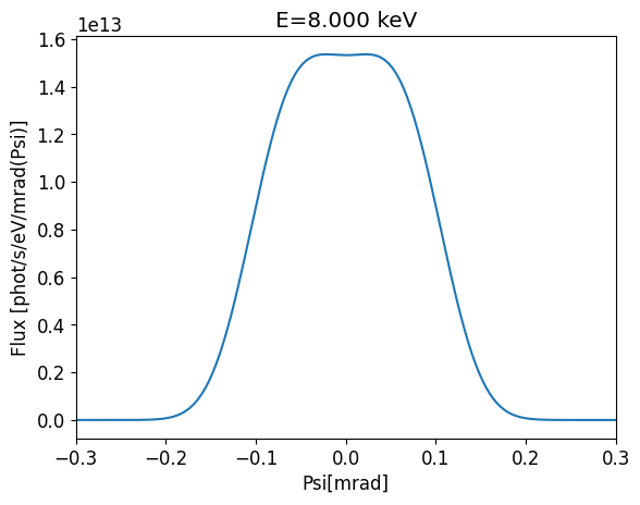
def check_esrf_bm_angle_flux_8keV(pltOk=False, method=1):
from srxraylib.sources.srfunc import sync_ang, sync_ene, sync_f
print("#")
print("# example 5: ESRF1 BM angular emission of flux")
print("#")
# input for ESRF1
energy = 8000.0
e_gev = 6.04 # electron energy in GeV
r_m = 25.0 # magnetic radius in m
i_a = 0.2 # electron current in A
# calculate critical energy in eV
codata_mee = 1e-6 * codata.m_e * codata.c ** 2 / codata.e
m2ev = codata.c * codata.h / codata.e # lambda(m) = m2eV / energy(eV)
gamma = e_gev*1e3/codata_mee
ec_m = 4.0*numpy.pi*r_m/3.0/numpy.power(gamma,3) # wavelength in m
ec_ev = m2ev/ec_m
npoints = 501
angle_mrad = numpy.linspace(-1.0, 1.0, npoints) # angle grid
flag = 1 # at at given energy
polarization = 0
if method ==0:
fluxEc = sync_ang(flag,angle_mrad,polarization=polarization, \
e_gev=e_gev,i_a=i_a,hdiv_mrad=1.0,energy=energy, ec_ev=ec_ev)
elif method == 1: # using eq in shadow4 paper
N0 = sync_ene(1, energy, ec_ev=ec_ev, polarization=0, e_gev=e_gev, i_a=i_a, hdiv_mrad=1.0,
psi_min=0.0, psi_max=0.0, psi_npoints=1)
F0 = sync_f(0, energy / ec_ev, polarization=1)
fluxEc = N0 / F0 * (
sync_f(angle_mrad * 1e-3 * gamma, energy / ec_ev, polarization=0) )
toptitle = "ESRF1 Bending Magnet angular emission 8 keV"
xtitle = "Psi[mrad]"
ytitle = "Flux [phot/s/0.1%bw/mrad(Psi)]"
if pltOk:
from srxraylib.plot.gol import plot
plot(angle_mrad, fluxEc, title="E=%.3f keV"%(energy*1e-3), xrange=[-0.3, 0.3], xtitle="Psi[mrad]", ytitle="Flux [phot/s/0.1%bw/mrad(Psi)]",
show=0)
plot(angle_mrad, fluxEc / (0.001 * energy), title="E=%.3f keV" % (energy * 1e-3), xrange=[-0.3, 0.3],
xtitle="Psi[mrad]", ytitle="Flux [phot/s/eV/mrad(Psi)]", show=0)
else:
print("\n\n\n\n\n######### %s ######### "%(toptitle))
print("\n %s %s "%(xtitle,ytitle))
for i in range(len(fluxEc)):
print(" %f %f"%(angle_mrad[i],fluxEc[i]))
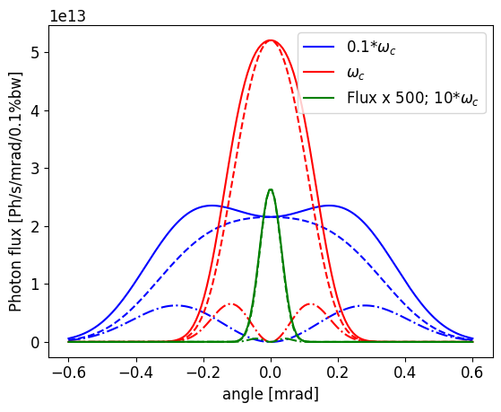
def check_clarke_43(pltOk=False):
from srxraylib.sources.srfunc import sync_ene
from mpl_toolkits.mplot3d import Axes3D # need for example 6
print("#")
print("# Example 6 Slide 35 of")
print("# http:https://www.cockcroft.ac.uk/wp-content/uploads/2014/12/Lecture-1.pdf")
print("#")
def calcFWHM(h,binSize):
t = numpy.where(h>=max(h)*0.5)
return binSize*(t[0][-1]-t[0][0]+1), t[0][-1], t[0][0]
#
e_gev = 3.0 # electron energy in GeV
b_t = 1.4 # magnetic radius in m
i_a = 0.3 # electron current in A
codata_mee = 1e-6 * codata.m_e * codata.c ** 2 / codata.e
gamma = e_gev*1e3/codata_mee
#calculates Magnetic radius
#cte = codata.m_e*codata.c/codata.e*(1/(codata_mee*1e-3)) # 0.3
#r_m = cte*e_gev/b_t
#more exactly
r_m = codata.m_e*codata.c/codata.e/b_t*numpy.sqrt( gamma*gamma - 1)
# calculate critical energy in eV
ec_m = 4.0*numpy.pi*r_m/3.0/numpy.power(gamma,3) # wavelength in m
m2ev = codata.c * codata.h / codata.e # lambda(m) = m2eV / energy(eV)
ec_ev = m2ev/ec_m
print("Gamma: %f \n"%(gamma))
print("Critical wavelength [A]: %f \n"%(1e10*ec_m))
print("Critical photon energy [eV]: %f \n"%(ec_ev))
e = numpy.array([0.1*ec_ev,ec_ev,10*ec_ev])
a = numpy.linspace(-0.6,0.6,150)
fm = sync_ene(4,e,ec_ev=ec_ev,e_gev=e_gev,i_a=i_a,\
hdiv_mrad=1,psi_min=-0.6,psi_max=0.6,psi_npoints=150)
fmPar = sync_ene(4,e,ec_ev=ec_ev,e_gev=e_gev,i_a=i_a,\
hdiv_mrad=1,psi_min=-0.6,psi_max=0.6,psi_npoints=150,polarization=1)
fmPer = sync_ene(4,e,ec_ev=ec_ev,e_gev=e_gev,i_a=i_a,\
hdiv_mrad=1,psi_min=-0.6,psi_max=0.6,psi_npoints=150,polarization=2)
toptitle='Flux vs vertical angle '
xtitle ='angle [mrad]'
ytitle = "Photon flux [Ph/s/mrad/0.1%bw]"
print("for E = 0.1 Ec FWHM=%f mrad "%( calcFWHM(fm[:,0],a[1]-a[0])[0]))
print("for E = Ec FWHM=%f mrad "%( calcFWHM(fm[:,1],a[1]-a[0])[0]))
print("for E = 10 Ec FWHM=%f mrad "%( calcFWHM(fm[:,2],a[1]-a[0])[0]))
print("Using approximated formula: ")
print("for E = 0.1 Ec FWHM=%f mrad "%( 0.682 / e_gev * numpy.power(10.0,0.425) ))
print("for E = Ec FWHM=%f mrad "%( 0.682 / e_gev * numpy.power(1.0,0.425) ))
print("for E = 10 Ec FWHM=%f mrad "%( 0.682 / e_gev * numpy.power(0.1,0.425) ))
if pltOk:
plt.figure(61)
ax = plt.subplot(111)
plt.plot(a,fm[:,0],'b', label="0.1*$\omega_c$")
plt.plot(a,fmPar[:,0],"b--")
plt.plot(a,fmPer[:,0],"b-.")
plt.xlabel(xtitle)
plt.ylabel(ytitle)
plt.figure(61)
plt.plot(a,fm[:,1],'red', label="$\omega_c$")
plt.plot(a,fmPar[:,1],"r--")
plt.plot(a,fmPer[:,1],"r-.")
plt.xlabel(xtitle)
plt.ylabel(ytitle)
factor = 500
plt.figure(61)
plt.plot(a, factor * fm[:,2],'green', label="Flux x %d; 10*$\omega_c$" % factor)
plt.plot(a, factor * fmPar[:,2],"g--")
plt.plot(a, factor * fmPer[:,2],"g-.")
plt.xlabel(xtitle)
plt.ylabel(ytitle)
legend_position = None
ax.legend(bbox_to_anchor=legend_position)
else:
print("\n\n\n\n\n######### %s ######### "%(toptitle))
print("\n %s %s %s "%(ytitle,xtitle,"Flux"))
for j in range(len(e)):
for i in range(len(a)):
print(" %f %f %e "%(e[j],a[i],fm[i,j]))
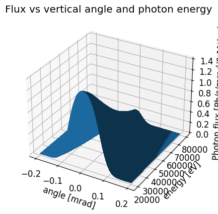
def check_esrf_bm_2d(pltOk=False):
from srxraylib.sources.srfunc import sync_ene
print("#")
print("# Example 7, ESRF1 flux vs energy and angle")
print("#")
# input for ESRF1
e_gev = 6.04 # electron energy in GeV
r_m = 25.0 # magnetic radius in m
i_a = 0.2 # electron current in A
# calculate critical energy in eV
codata_mee = 1e-6 * codata.m_e * codata.c ** 2 / codata.e
gamma = e_gev*1e3/codata_mee
ec_m = 4.0*numpy.pi*r_m/3.0/numpy.power(gamma,3) # wavelength in m
m2ev = codata.c * codata.h / codata.e # lambda(m) = m2eV / energy(eV)
ec_ev = m2ev/ec_m
a = numpy.linspace(-0.2,0.2,50)
e = numpy.linspace(20000,80000,80)
fm = sync_ene(4,e,ec_ev=ec_ev,e_gev=e_gev,i_a=i_a,\
hdiv_mrad=1,psi_min=a.min(),psi_max=a.max(),psi_npoints=a.size)
toptitle='Flux vs vertical angle and photon energy'
xtitle ='angle [mrad]'
ytitle ='energy [eV]'
ztitle = "Photon flux [Ph/s/mrad/0.1%bw]"
if pltOk:
fig = plt.figure(7)
ax = fig.add_subplot(111, projection='3d')
fa, fe = numpy.meshgrid(a, e)
surf = ax.plot_surface(fa, fe, fm.T, \
rstride=1, cstride=1, \
linewidth=0, antialiased=False)
plt.title(toptitle)
ax.set_xlabel(xtitle)
ax.set_ylabel(ytitle)
ax.set_zlabel(ztitle)
else:
print("\n\n\n\n\n######### %s ######### "%(toptitle))
print("\n %s %s %s "%(xtitle,ytitle,ztitle))
for i in range(len(a)):
for j in range(len(e)):
print(" %f %f %e "%(a[i],e[j],fm[i,j]))
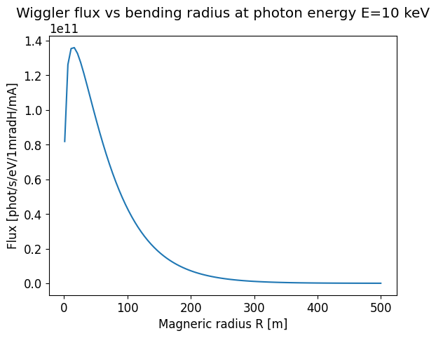
def check_wiggler_flux_vs_r(pltOk=False):
from srxraylib.sources.srfunc import wiggler_nphoton
print("#")
print("# Example 8 (Wiggler flux vs bending radius at a given photon energy)")
print("#")
r_m = numpy.linspace(1.0,500.0,100)
flux = wiggler_nphoton(r_m,electronEnergy=6.04,photonEnergy=10000.0)
toptitle = "Wiggler flux vs bending radius at photon energy E=10 keV"
xtitle = "Magneric radius R [m]"
ytitle = "Flux [phot/s/eV/1mradH/mA]"
if pltOk:
plt.figure(8)
plt.plot(r_m,flux)
plt.title(toptitle)
plt.xlabel(xtitle)
plt.ylabel(ytitle)
else:
print("\n\n\n\n\n######### %s ######### "%(toptitle))
print("\n %s %s "%(xtitle,ytitle))
for i in range(len(r_m)):
print(" %f %e"%(r_m[i],flux[i]))
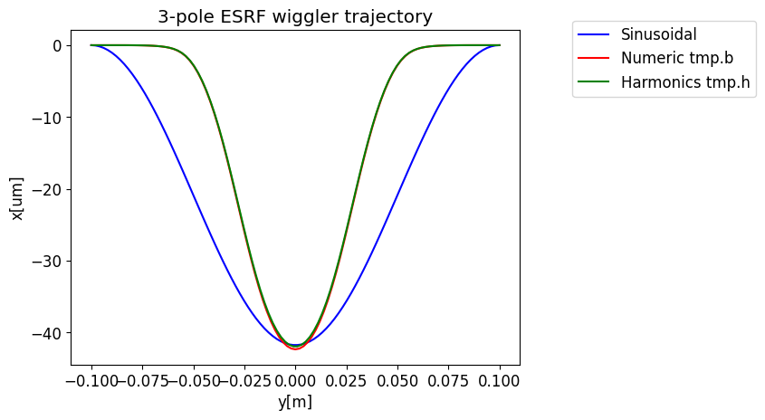
def check_wiggler_external_b(pltOk=False):
from srxraylib.sources.srfunc import wiggler_trajectory, wiggler_spectrum, wiggler_harmonics
print("#")
print("# Example 9 (Wiggler trajectory and flux for a 3pole wiggler ")
print("#")
# this is the B(s) map (T, m)
b_t = numpy.array([[ -1.00000000e-01, 1.08200000e-03],
[ -9.80000000e-02, 8.23000000e-04],
[ -9.60000000e-02, 4.45000000e-04],
[ -9.40000000e-02, 8.60000000e-05],
[ -9.20000000e-02, -4.93000000e-04],
[ -9.00000000e-02, -1.20800000e-03],
[ -8.80000000e-02, -2.16100000e-03],
[ -8.60000000e-02, -3.44500000e-03],
[ -8.40000000e-02, -5.10500000e-03],
[ -8.20000000e-02, -7.34500000e-03],
[ -8.00000000e-02, -1.03050000e-02],
[ -7.80000000e-02, -1.42800000e-02],
[ -7.60000000e-02, -1.96770000e-02],
[ -7.40000000e-02, -2.70560000e-02],
[ -7.20000000e-02, -3.73750000e-02],
[ -7.00000000e-02, -5.20600000e-02],
[ -6.80000000e-02, -7.35170000e-02],
[ -6.60000000e-02, -1.05680000e-01],
[ -6.40000000e-02, -1.54678000e-01],
[ -6.20000000e-02, -2.28784000e-01],
[ -6.00000000e-02, -3.34838000e-01],
[ -5.80000000e-02, -4.70272000e-01],
[ -5.60000000e-02, -6.16678000e-01],
[ -5.40000000e-02, -7.46308000e-01],
[ -5.20000000e-02, -8.39919000e-01],
[ -5.00000000e-02, -8.96470000e-01],
[ -4.80000000e-02, -9.26065000e-01],
[ -4.60000000e-02, -9.38915000e-01],
[ -4.40000000e-02, -9.40738000e-01],
[ -4.20000000e-02, -9.32236000e-01],
[ -4.00000000e-02, -9.08918000e-01],
[ -3.80000000e-02, -8.60733000e-01],
[ -3.60000000e-02, -7.73534000e-01],
[ -3.40000000e-02, -6.36577000e-01],
[ -3.20000000e-02, -4.52611000e-01],
[ -3.00000000e-02, -2.37233000e-01],
[ -2.80000000e-02, -7.09700000e-03],
[ -2.60000000e-02, 2.26731000e-01],
[ -2.40000000e-02, 4.54558000e-01],
[ -2.20000000e-02, 6.61571000e-01],
[ -2.00000000e-02, 8.29058000e-01],
[ -1.80000000e-02, 9.45984000e-01],
[ -1.60000000e-02, 1.01683300e+00],
[ -1.40000000e-02, 1.05536200e+00],
[ -1.20000000e-02, 1.07490000e+00],
[ -1.00000000e-02, 1.08444200e+00],
[ -8.00000000e-03, 1.08898000e+00],
[ -6.00000000e-03, 1.09111200e+00],
[ -4.00000000e-03, 1.09208300e+00],
[ -2.00000000e-03, 1.09249400e+00],
[ 0.00000000e+00, 1.09262000e+00],
[ 2.00000000e-03, 1.09249400e+00],
[ 4.00000000e-03, 1.09208300e+00],
[ 6.00000000e-03, 1.09111200e+00],
[ 8.00000000e-03, 1.08898000e+00],
[ 1.00000000e-02, 1.08444200e+00],
[ 1.20000000e-02, 1.07490000e+00],
[ 1.40000000e-02, 1.05536200e+00],
[ 1.60000000e-02, 1.01683300e+00],
[ 1.80000000e-02, 9.45984000e-01],
[ 2.00000000e-02, 8.29058000e-01],
[ 2.20000000e-02, 6.61571000e-01],
[ 2.40000000e-02, 4.54558000e-01],
[ 2.60000000e-02, 2.26731000e-01],
[ 2.80000000e-02, -7.09700000e-03],
[ 3.00000000e-02, -2.37233000e-01],
[ 3.20000000e-02, -4.52611000e-01],
[ 3.40000000e-02, -6.36577000e-01],
[ 3.60000000e-02, -7.73534000e-01],
[ 3.80000000e-02, -8.60733000e-01],
[ 4.00000000e-02, -9.08918000e-01],
[ 4.20000000e-02, -9.32236000e-01],
[ 4.40000000e-02, -9.40738000e-01],
[ 4.60000000e-02, -9.38915000e-01],
[ 4.80000000e-02, -9.26065000e-01],
[ 5.00000000e-02, -8.96470000e-01],
[ 5.20000000e-02, -8.39919000e-01],
[ 5.40000000e-02, -7.46308000e-01],
[ 5.60000000e-02, -6.16678000e-01],
[ 5.80000000e-02, -4.70272000e-01],
[ 6.00000000e-02, -3.34838000e-01],
[ 6.20000000e-02, -2.28784000e-01],
[ 6.40000000e-02, -1.54678000e-01],
[ 6.60000000e-02, -1.05680000e-01],
[ 6.80000000e-02, -7.35170000e-02],
[ 7.00000000e-02, -5.20600000e-02],
[ 7.20000000e-02, -3.73750000e-02],
[ 7.40000000e-02, -2.70560000e-02],
[ 7.60000000e-02, -1.96770000e-02],
[ 7.80000000e-02, -1.42800000e-02],
[ 8.00000000e-02, -1.03050000e-02],
[ 8.20000000e-02, -7.34500000e-03],
[ 8.40000000e-02, -5.10500000e-03],
[ 8.60000000e-02, -3.44500000e-03],
[ 8.80000000e-02, -2.16100000e-03],
[ 9.00000000e-02, -1.20800000e-03],
[ 9.20000000e-02, -4.93000000e-04],
[ 9.40000000e-02, 8.60000000e-05],
[ 9.60000000e-02, 4.45000000e-04],
[ 9.80000000e-02, 8.23000000e-04],
[ 1.00000000e-01, 1.08200000e-03]])
# normal (sinusoidal) wiggler
t0,p = wiggler_trajectory(b_from=0, nPer=1, nTrajPoints=100, \
ener_gev=6.04, per=0.2, kValue=7.75, \
trajFile="tmpS.traj")
# magnetic field from B(s) map
t1,p = wiggler_trajectory(b_from=1, nPer=1, nTrajPoints=100, \
ener_gev=6.04, inData=b_t,trajFile="tmpB.traj")
# magnetic field from harmonics
hh = wiggler_harmonics(b_t,Nh=41,fileOutH="tmp.h")
t2,p = wiggler_trajectory(b_from=2, nPer=1, nTrajPoints=100, \
ener_gev=6.04, per=0.2, inData=hh,trajFile="tmpH.traj")
toptitle = "3-pole ESRF wiggler trajectory"
xtitle = "y[m]"
ytitle = "x[um]"
if pltOk:
plt.figure(91)
plt.plot(t0[1,:],1e6*t0[0,:],'b',label="Sinusoidal")
plt.plot(t1[1,:],1e6*t1[0,:],'r',label="Numeric tmp.b")
plt.plot(t2[1,:],1e6*t2[0,:],'g',label="Harmonics tmp.h")
plt.title(toptitle)
plt.xlabel(xtitle)
plt.ylabel(ytitle)
ax = plt.subplot(111)
ax.legend(bbox_to_anchor=(1.1, 1.05))
else:
print("\n\n\n\n\n######### %s ######### "%(toptitle))
print(" x[m] y[m] z[m] BetaX BetaY BetaZ Curvature B[T] ")
for i in range(t2.shape[1]):
print(("%.2e "*8+"\n")%( tuple(t2[0,i] for i in range(t2.shape[0]) )))
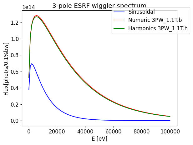
if True:
#
# now spectra
#
e, f0, tmp = wiggler_spectrum(t0,enerMin=100.0,enerMax=100000.0,nPoints=100, \
electronCurrent=0.2, outFile="tmp.dat", elliptical=False)
e, f1, tmp = wiggler_spectrum(t1,enerMin=100.0,enerMax=100000.0,nPoints=100, \
electronCurrent=0.2, outFile="tmp.dat", elliptical=False)
e, f2, tmp = wiggler_spectrum(t2,enerMin=100.0,enerMax=100000.0,nPoints=100, \
electronCurrent=0.2, outFile="tmp.dat", elliptical=False)
toptitle = "3-pole ESRF wiggler spectrum"
xtitle = "E [eV]"
ytitle = "Flux[phot/s/0.1%bw]"
if pltOk:
plt.figure(92)
plt.plot(e,f0,'b',label="Sinusoidal")
plt.plot(e,f1,'r',label="Numeric 3PW_1.1T.b")
plt.plot(e,f2,'g',label="Harmonics 3PW_1.1T.h")
plt.title(toptitle)
plt.xlabel(xtitle)
plt.ylabel(ytitle)
ax = plt.subplot(111)
ax.legend(bbox_to_anchor=(1.1, 1.05))
else:
print("\n\n\n\n\n######### %s ######### "%(toptitle))
print(" energy[eV] flux_sinusoidal flux_fromB flux_fromHarmonics ")
for i in range(t2.shape[1]):
print(("%.2e "*4+"\n")%( e[i],f0[i], f1[i], f2[i] ))
def check_wiggler_polarization(pltOk=False):
from srxraylib.sources.srfunc import wiggler_trajectory, wiggler_spectrum
print("#")
print("# Example 10 (Wiggler flux vs polarization)")
print("#")
t0, p = wiggler_trajectory(b_from=0, nPer=37, nTrajPoints=1001, \
ener_gev=3.0, per=0.120, kValue=22.416, \
trajFile="")
e, f0, p0 = wiggler_spectrum(t0, enerMin=100, enerMax=100100, nPoints=500, \
electronCurrent=0.1, outFile="", elliptical=False, polarization=0)
e, f1, p1 = wiggler_spectrum(t0, enerMin=100, enerMax=100100, nPoints=500, \
electronCurrent=0.1, outFile="", elliptical=False, polarization=1)
e, f2, p2 = wiggler_spectrum(t0, enerMin=100, enerMax=100100, nPoints=500, \
electronCurrent=0.1, outFile="", elliptical=False, polarization=2)
toptitle = "Wiggler flux vs polarization"
xtitle = "Photon energy [eV]"
ytitle = "Flux [phot/s]"
if pltOk:
plt.figure(10)
plt.plot(e, f0)
plt.plot(e, f1)
plt.plot(e, f2)
# plt.plot(e, f1 + f2)
plt.title(toptitle)
plt.xlabel(xtitle)
plt.ylabel(ytitle)
else:
print("\n\n\n\n\n######### %s ######### "%(toptitle))
print("\n %s %s "%(xtitle,ytitle))
for i in range(len(e)):
print(" %f %e"%(e[i],f0[i]))
def check_shadow4(pltOk=False):
import time
from srxraylib.sources.srfunc import sync_f_sigma_and_pi, sync_f_sigma_and_pi_approx, kv_approx
from scipy.special import kv, gamma
if True:
# test speed
psi1 = 0.0
psi_interval_number_of_points = 1001
angle_array_reduced = numpy.linspace(-0.5 * psi1, 0.5 * psi1, psi_interval_number_of_points)
t0 = time.time()
for i in range(15000):
tmp = sync_f_sigma_and_pi(angle_array_reduced, 100.)
print("Time (accurate): ", time.time()-t0)
t0 = time.time()
for i in range(15000):
tmp = sync_f_sigma_and_pi_approx(angle_array_reduced, 100.)
print("Time (approximated): ", time.time()-t0)
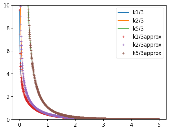
if True:
# display/compare Kv approximated
ji_interval_number_of_points = 1001
ji_array = numpy.linspace(0, 5, ji_interval_number_of_points)
k13 = kv(1.0 / 3.0, ji_array)
k23 = kv(2.0 / 3.0, ji_array)
k53 = kv(5.0 / 3.0, ji_array)
k13approx = kv_approx(1.0 / 3.0, ji_array)
k23approx = kv_approx(2.0 / 3.0, ji_array)
k53approx = kv_approx(5.0 / 3.0, ji_array)
from srxraylib.plot.gol import plot
plot(ji_array, k13,
ji_array, k23,
ji_array, k53,
ji_array, k13approx,
ji_array, k23approx,
ji_array, k53approx,
legend=['k1/3','k2/3','k5/3', 'k1/3approx','k2/3approx','k5/3approx'],
marker=[None, None, None, '+', '+', '+'], linestyle=[None,None,None,'','',''], xlog=0, ylog=0, yrange=[1e-18,10],
show=pltOk)
if True:
# test flatness (wiggler interpolation error).
psi1 = 50.0
psi_interval_number_of_points = 1001
angle_array_reduced = numpy.linspace(-0.5 * psi1, 0.5 * psi1, psi_interval_number_of_points)
eene = numpy.linspace(1, 1e4, 100)
t0 = time.time()
for i in range(eene.size):
fm_s, fm_p = sync_f_sigma_and_pi(angle_array_reduced, eene[i])
print(eene[i], fm_s.min(), fm_s.max(), fm_s.max() - fm_s.min())
def check_constants():
from srxraylib.sources.srfunc import sync_ene, sync_hi, sync_g1, sync_ang, sync_ene
cte0 = sync_ene(1, 1000.0, ec_ev=1000.0, polarization=0, e_gev=1.0, i_a=1.0, hdiv_mrad=1.0,
psi_min=0.0, psi_max=0.0, psi_npoints=1)
h2 = sync_hi(1.0, i=2, polarization=1)
print("cte0 (for flux on axis): %g cte0*h2: %g " % (cte0 / h2, cte0))
cte1 = sync_ene(0, 10000.0, ec_ev=10000.0, polarization=0, e_gev=1.0, i_a=1.0, hdiv_mrad=1.0,
psi_min=0.0, psi_max=0.0, psi_npoints=1)
g1 = sync_g1(1.0)
cte1 = cte1 / g1
print("cte1 (for flux integrated in psi): %g" % cte1)
#
#------------------------- MAIN ------------------------------------------------
#
if __name__ == '__main__':
pltOk = True
check_xraybooklet_fig2_1(pltOk=pltOk)
check_xraybooklet_fig2_2(pltOk=pltOk)
check_esrf_bm_spectrum(pltOk=pltOk)
check_esrf_bm_angle_power(pltOk=pltOk)
check_esrf_bm_angle_flux(pltOk=pltOk, method=0)
check_esrf_bm_angle_flux_8keV(pltOk=pltOk, method=0)
check_esrf_bm_angle_flux(pltOk=pltOk, method=1)
check_clarke_43(pltOk=pltOk)
check_esrf_bm_2d(pltOk=pltOk)
check_wiggler_flux_vs_r(pltOk=pltOk)
check_wiggler_external_b(pltOk=pltOk)
# # check_wiggler_polarization(pltOk=pltOk) # slow
check_shadow4(pltOk=pltOk)
check_constants()
if pltOk: plt.show()